Shadow and Solar Panels: a Short Analysis

In these strange times of lockdown and curfew, I have some extra time on my hands. Combined with my background in physics and my desire to understand technical things, this has resulted in a number of toy projects in which I attempt to measure something not-so-useful. This is one of those projects.

My Solar Panels

Just over a year ago I moved into a newly built house. The house came with a set of solar panels. This is nothing special – in the Netherlands solar panels are requirement to obtain a building permit nowadays. The building permit is rather specific about it: it lists the number of panels, their location ("on the roof"), their orientation ("West"), their angle with respect to horizontal (56 degrees), as well as the amount of shadow ("minimal"). Interestingly, the panels are mounted on the Eastern side of the rather steep gable roof of my house – not the Western side like the permit specifies. This is even more interesting because the neighboring house on the Eastern side lies much closer to our house than the house on the Western side – close enough to cast a shadow on the panels. I cannot help but wonder why they decided to mount the panels facing East – and whether the effect of the shadow of the neighboring house is indeed "minimal".

Finding the person who installed the solar panels on my house – in order to ask them why they chose the other side of the roof – is going to be difficult, but I can estimate the impact of the shadow on the yield.

Obtaining Data

The journey of any data science project, even toy projects, starts with gathering data. First, let’s have a look at the panels themselves: they are hooked up to a Zeverlution 2000S inverter. When connected to WiFi or an ethernet cable, this inverter provides a REST API that can tell you the current power (in Watt), the total energy yield of today (in kWh), and the current time in China. I currently do have a setup that polls this API every 30 seconds and stores it in InfluxDB, but this has only been running for a couple of months now. A better source is the Zevercloud – the cloud service that the Zeverlution automatically reports its statistics to since it was installed. So this invasion of privacy has a benefit after all!

Zevercloud does not have any functionality to export any data, but we can find plots of the yield of the panels on any given day in the past. For example the 5th of March this year, which was a beautiful day:

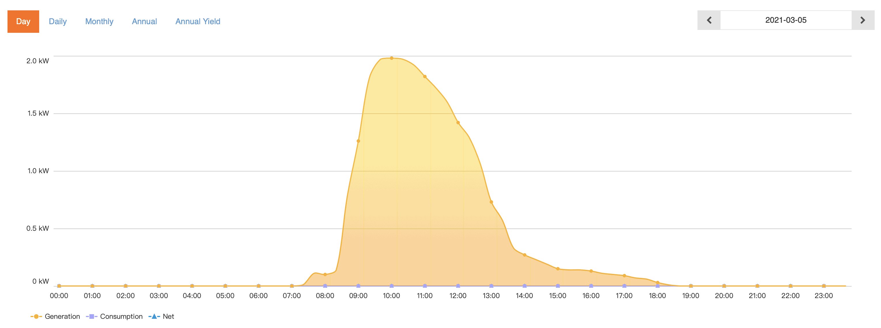
Luckily this plot is generated client-side, which means that there is an API that we can query to extract the data that we need. After looking up the cookies my browser uses for authentication, I was able to get the full day’s worth of data (in 10 minute intervals) in somewhat strangely structured, but useable, JSON format:

{
  ...
  "unit": "kW",
  "qdate": "2021-03-05",
  "dataset": [
    ...
    {
      "time" : "07:40",
      "value" : [ "0.10" ],
      "consump" : 0.0,
      "mexport" : 0.0,
      "mimport" : 0.0,
      "net" : 0.0
      }, {
      "time" : "08:00",
      "value" : [ "0.21" ],
      "consump" : 0.0,
      "mexport" : 0.0,
      "mimport" : 0.0,
      "net" : 0.0
      },
      ...
  ]
}

Here the time is even converted to my time zone (but ignoring summer time altogether). If I can do this once, then I can do this many times! So a script that does this for every day since the beginning of time (i.e. beginning of time for this inverter, which is just over a year ago) was quickly written.

Next, I needed to convert this a better format (a flat table), and to fix the time zone. And while I was at it: join it with weather data for the area obtained from the KNMI.

Enriching the Data

In addition to the timestamp and the instantaneous power yield of the inverter, we need to know the position of the sun on the sky.
We define this position by the altitude (degrees above the horizon) and the azimuth (in degrees with respect to due South), and it
can easily be calculated using soltrack. Another useful feature is the angle
of the sun with respect to the solar panels: the incidence angle, which is equal to zero when the sun is exactly perpendicular to the panels.
In my case, this is when the sun is at an altitude of 34 degrees, and an azimuth of -84 degrees (6 degrees South of due East). Also interesting is the cosine of this angle, the incidence factor, which describes the direct radiation from the sun on the panel.

Exploration

Now let’s have a look at the data. Here is a figure with a number of power curves (the power is normalized to the peak power of all panels) for a number of days across the year:

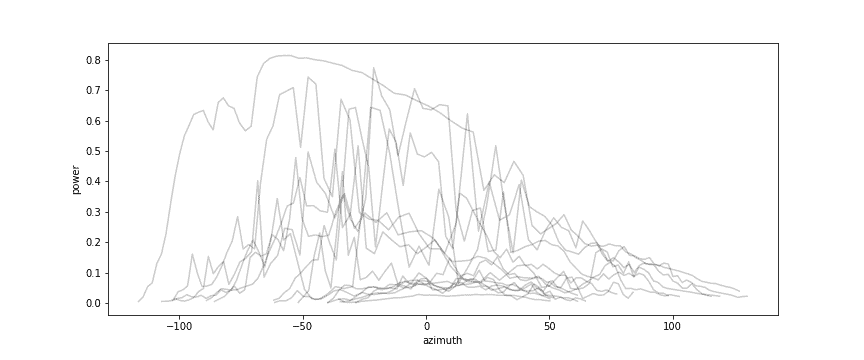
We can clearly see the difference between winter and summer days, we see that not a single day has a smooth curve (welcome to Dutch weather). We can also clearly see that the power is higher in the morning (azimuth < 0) – which makes sense because the panels are facing East.

Here is another interesting plot:

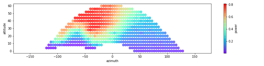
It shows the maximum power recorded in each segment of the sky – taking the maximum gets rid of (most) cloudy data. We can clearly see the silhouette of the neighboring house, which has a gable roof that is rotated 90 degrees: we are looking at one end. At the bar on the right we can see that the yield never goes beyond roughly 80% of the peak power: the limiting factor here is the inverter. It is common practice to under-dimension the inverter to save costs.

Modeling

Next we’ll try to model the power output of the solar panels as a function of the location of the sun. In order to keep it simple we’ll first only look at data from moments at which the sky was clear – according to the KNMI. Below is a plot of the incidence factor versus the power output. As we expect the power increases with the incidence factor: more sunlight on the panels means more power.

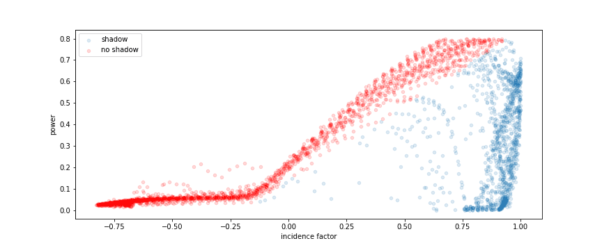
On the right we see quite a few points that are below the trend line – I’ve marked them blue. This is where the solar panels are in the shadow of the other house. We will ignore these points for now. I have also removed all points where the inverter was at its limit: these points would introduce a non-linearity I’d rather not deal with.

Indirect Light

On the left of the plot above we see that even if there is no direct sunlight on the solar panels (the incidence factor < 0), there is still some power yield. This comes from indirect sunlight, reflected by the sky or some object. We do see that this goes down at the far end, where the sun nearly sets. It turns out that this indirect power can be modeled fairly accurately using only the altitude: if the sun is high in the sky, there is more indirect light.

The figure below, on the left, shows a scatter plot of the power versus the insolence, which is the cosine of the altitude of the sun.

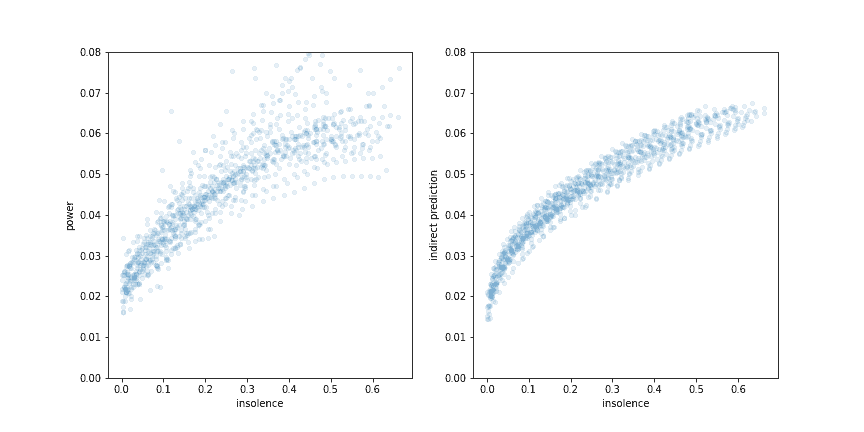
The results on the right are from a statsmodels OLS fit of the following model: power ~ insolence + np_sqrt(insolence) + temperature.
Interestingly, the temperature coefficient comes out as -0.00037, which is very close to the -0.000365 the manufacturer specifies! We may be doing something that actually makes sense!

Direct Light

Even when there is direct sunlight on a solar panel, part of the generated power will come from indirect light. If we assume this part to be independent
of the incidence angle, we can compute the contribution from direct light by estimating the contribution from indirect light using the model above,
and subtracting that from the actual power.

Naively one might expect the contribution of direct light to be zero when the incidence factor equals zero, but it appears that the effect "direct" light starts kicking in when the incidence factor is around -0.13, as can be seen in the plot below.

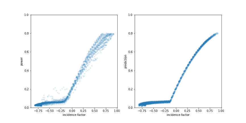
Again the results on the right are from a statsmodels OLS fit, this time on the model direct ~ incidence_factor_cutoff + np_power(incidence_factor_cutoff, 2) + temperature, where direct is the power minor the indirect component, and incidence_factor_cutoff is the incidence factor minus the cutoff (-0.13).

Modeling Shadow

Now that we have a model describing the power yield of the solar panels in an ideal situation (with a clear sky, no shadow), we can
use that to make a model of the shadow. We define power / predicted_power as a measure for shadow – of course taking only data with
a clear sky – and train a random forest to predict the shadow as a function of azimuth and altitude. This is the result:

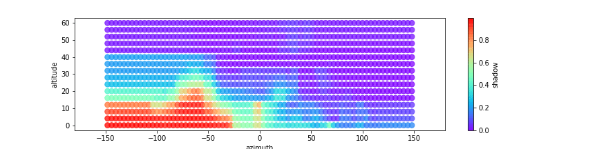
Again we can clearly see the silhouette of the neighboring house, as well as a little bit of shadow caused by the exhaust of the ventilation system immediately South of the solar panels.

The Effect of Shadow

Now we can get an estimate of the effect of the shadow on the total yield of the solar panels: by simply comparing the integral of the power with the integral of the predicted power, I find a difference of roughly 250 kWh over the course of last year. But note that this is only on the sunny moments!
Using the model for shadow, we can repeat the analysis for cloudy moments. The results aren’t as good a fit, of course, but in the end the model describes the data pretty well. Again comparing power with predicted power, I find a difference of another 450kWh! I would not call that "minimal"!

Conclusion

It turns out that the power yield of a solar panel isn’t too difficult to model using only altitude, incidence angle, temperature and cloudiness as variables. It also turns out that if whoever installed my solar panels had decided to do so on the other side of my house, these panels would have yielded an estimated 170 euro per year more.

If you are interested in the code of this analysis, have a look here.