How to style transfer your own images

Inspired by Gene Kogan’s keynote at PyData Warsaw 2018, we decided to dive into style transferring ourselves during our fast.ai pressure cooker last December. This blog explains what it is and describes two approaches on how to do it yourself.

The term “style transfer” is used to describe the operation of recomposing one image in the style of another (group of) image(s). In general, this requires two inputs: content image(s) and style image(s). The technique applied should then produce output whose “content” mirrors the content image and whose “style” resembles that of the style image.

Below an example with an original cat photo on the left (the content image), which is “styled” in three different ways using the style images in the middle. The different styles lead to different generated output images, as can be seen on the right.

Diving into this topic we found multiple ways to do style transfer. We will share two approaches here, including code so you can create your own styled images.

Approach 1: Neural Style

Neural style transfer was first demonstrated in August 2015 in a paper published by Gatys, Ecker, and Bethge at the University of Tübingen. The algorithm is described well on ml4a, a website by Gene Kogan that provides free educational resources about machine learning for artists.

In short, the objective of the style transfer algorithm is to generate an output image which minimizes a loss function that is the sum of two separate terms, a “content loss” and a “style loss.” The content loss represents the dissimilarity between the content image and the output image, whereas the style loss represents dissimilarity between the style image and the output image.

The algorithm trains a single convolutional neural network, wherein at each iteration the output image’s pixels are slightly adjusted so as to decrease the overall loss. We do this repeatedly until the loss converges, or until we are satisfied with our result.

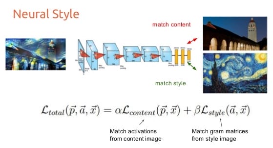
The content and style loss are defined differently:

• For the content loss the output image and content image are run through the convnet, giving us a set of feature maps for both. The loss at a single layer is then the euclidean (L2) distance between the activations of the content image and the activations of the output image.
• For the style loss we also use the convnet’s activations, but instead of comparing the raw activations directly, we take the Gram matrix of the activations at each layer in the network. This is a way to capture correlations between features in different parts of the image, which turns out to be a very good representation of our perception of style within images. The style loss at a single layer is then defined as the euclidean (L2) distance between the Gram matrices of the style and output images.

When running this model for a content image of Amsterdam and a winter-theme style image, we get a pretty neat result!

Note that our style image is not really a style, but more a winter-theme picture. The textures in the style images from the cat examples in the introduction are much easier to transfer. However, in our case, you can still clearly see that the model has picked up on the branch structure of the trees.

Read the appendix below for instructions on how to run this yourself.

Approach 2: Cycle-Consistent Adversarial Networks

The second approach we used is based on this recent paper and its implementation. It’s called Unpaired Image-to-Image Translation using Cycle-Consistent Adversarial Networks. Instead of learning from paired examples (transform from picture X_i to picture Y_i) it learns from unpaired sets of data X and Y (transform a picture from X into style of Y). This is easier because getting paired data is often expensive and difficult.

The goal is to learn the transformation from X (content images) to Y’ such that Y’ looks as it’s from Y (style images). We can verify this with an adversarial model that tries to distinguish Y’ from Y.

A problem that might arise is that our transformation learns to always produce the same Y’ that is able to fool the adversarial model. To overcome this problem we want our model to be “cycle consistent”, that is we also want to learn a model to transfer Y’ back to X’ where X’ should be close to X again.

The image below gives a schematic overview of this approach. On the left (a) we see our models F and G which can style transfer images between X and Y. Further, we have D_X and D_Y which are the adversarial discriminators. D_X encourages F to translate Y into X’ outputs indistinguishable from domain X.

In the middle (b), we see the cycle-consistency loss which is used to make sure that the images transformed by G can be transformed back by F into something that resembles the original X. On the right (c) we see the same for transformations from Y to X and back to Y.

Using this approach on the same content (Amsterdam) and style (winter) images, we again get a very nice result. It is interesting to see how the different methods generate quite different output images. The content isn’t warped or skewed, only a lot of white is added which really give it a winter style. The thing that gives away that it’s a generated image is the white bottom and front side of the bridge is also white.

Want to try it yourself, check the appendix below on how to get everything running.

Wrap up

For our style transfer exercise we played around with two approaches. Where the first approach of neural style transfer is learning a mapping between two specific images, cycle-consistent adversarial networks can learn a mapping between two image collections (although in our Amsterdam-winter example each collection contained just a single picture). This second approach is more rich as it attempts to mimic the style of an entire collection of artworks, rather than transferring the style of a single selected piece of art. Therefore, cycle-consistent adversarial networks learn to generate photos in the style of, e.g., Van Gogh, rather than just in the style of Starry Night¹.

We hope this blog will help you get started with style transferring yourself. Have fun doing so!

Appendix

Approach 1: Set-up of Neural Style

To run the code yourself, clone and follow the instructions from this Torch neural-style project (written in Lua). If you feel more comfortable with Python, try out this tutorial for neural transfer using PyTorch. Torch is a separate product from PyTorch; PyTorch has no dependencies on Torch.

The instructions for the Torch tutorial are for Ubuntu (great when running in the cloud), so a little tweaking is required for running neural style on your mac. If you don’t have an nVidia GPU on your machine you can still run the code using your local machine’s CPU with the flag -gpu -1:

th neural_style.lua 
    -style_image examples/inputs/shipwreck.jpg 
    -content_image examples/inputs/golden_gate.jpg 
    -output_image examples/outputs/my_output_image.png 
    -gpu -1

Approach 2: Set-up of Cycle-Consistent Adversarial Networks

To get you own code running, follow the instructions below. First create a new conda environment and activate it:

conda create -n style-transfer
conda activate style-transfer  # or use source activate for older versions of conda

Clone this repository and to make sure you can reproduce our results, checkout a specific commit from December 2018:

git clone https://github.com/junyanz/pytorch-CycleGAN-and-pix2pix
cd pytorch-CycleGAN-and-pix2pix
git checkout c8323f9d0167161df1ad92e583f2a395fb59b5e8

Run a script to install the necessary packages and update everything:

bash ./scripts/conda_deps.sh
conda update --all

If you want to reproduce the horse to zebra results you can download a pre-trained model and the corresponding data (to be able to test the model) with the following scripts:

bash ./scripts/download_cyclegan_model.sh horse2zebra
bash ./datasets/download_cyclegan_dataset.sh horse2zebra

To generate the results for horse to zebra data run the following:

python test.py --dataroot datasets/horse2zebra/testA --name horse2zebra_pretrained--model test --gpu_ids -1 --no_dropout

Wherein these are the arguments we use:

• --dataroot: Path to the data set.
• --name: Name of the experiment. It decides where to store samples and models. Also tries to load ./checkpoints/{name}/latest_net_G.pth’
• --model: Specify the model to be used. We use TesteModel to generate CycleGAN results for only one direction. This model will automatically set --dataset_mode single, which only loads the images from one collection.
• --display_id: Set to -1 to avoid the extra overhead of communicating with visdom.
• --gpu_ids: Set to -1 to run locally without an NVIDIA GPU.
• --no_dropout: No dropout.
• --resize_or_crop: Set to none to keep original image size.

Running your own data set

To do the same for you own data set you first have to create a new folder in the datasets directory containing two folders trainA and trainB which hold images from two different groups (e.g. horses in A and zebras in B).

Then you train a new model which you use to transfer the style. First, learn the style transfer model by running (replace matrix with your own data set):

python train.py --dataroot ./datasets/matrix --name matrix_cyclegan --model cycle_gan --gpu_ids -1 --display_id -1

After training, transfer the style from trainB to all images from trainA, as follows:

python test.py --dataroot datasets/matrix/trainA --name matrix_cyclegan --model test --model_suffix "_A" --gpu_ids -1 --no_dropout --resize_or_crop none

To speed up the process you can spin up a GPU in the cloud and run the same code without the option --gpu_ids -1. For us this resulted in a speed up with factor 60; epochs taking 3 seconds rather than 3 minutes.

Want to do cool stuff like this yourself?

Our three-day course on Deep Learning dives into all aspects of deep learning, including image recognition and classification.