Graph partitioning in MapReduce with Cascading (part 1)

I have recently had the joy of doing MapReduce based graph partitioning. Here’s a post about how I did that. I decided to use Cascading for writing my MR jobs, as it is a lot less verbose than raw Java based MR. The graph algorithm consists of one step to prepare the input data and then a iterative part, that runs until convergence. The program uses a Hadoop counter to check for convergence and will stop iterating once there. All code is available. Also, the explanation has colorful images of graphs. (And everything is written very informally and there is no math.)
I have a graph and it looks like this (this graph is disconnected, but we will later on also partition fully connected graphs based on some partitioning criterion):

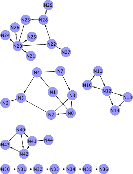
This is only true when you visualize the graph. In reality, it’s just a text file that contains a list of edges in the form of source and target node IDs. The above graph is this:

0,1
0,2
0,3
1,4
4,5
5,6
2,3
2,5
4,7
7,3
10,11
11,12
12,10
12,13
12,14
13,14
20,21
20,22
20,23
20,24
20,25
20,26
22,27
22,28
28,23
28,29
30,31
31,32
32,33
33,34
34,35
35,36
40,41
40,42
40,43
42,43
42,41
41,44

Now, what we aim to do is tag each edge in the list with a partition number. The graph is potentially very large and it will not fit in the memory of a single machine. This gives us an excuse to use MapReduce for the partitioning. Once it is partitioned, we can later on do analysis on the different parts of the graph independently and hopefully each partition will be small enough to fit in memory, so we can also visualize them.

The algorithm that we will apply is this:

Turn the edge lists into an adjacency list representation
Tag each source node + adjacency list with a partition ID equal to the largest node ID in the record. So partition ID = max(source node ID, target node IDs).
For each node ID, find the largest partition ID that it belongs to. So if a node is part of two or more adjacency lists, find the one that has the largest partition ID.
Set the partition ID of each record to the largest partition ID found in step 3
Repeat step 3 and 4 until nothing changes anymore.
We’ll go through this step by step. While we will be doing everything using MapReduce, we are using Cascading as a layer of abstraction over MapReduce. With Cascading, you don’t think in mappers and reducers, but in record processing using tuples. on which you apply functions, aggregates, grouping and joins. Writing raw MapReduce jobs is tedious, verbose and very time consuming. Unless you absolutely need to for performance or other reasons, writing bare MapReduce should be avoided in favor of some abstraction layer. There are many of these in a number of languages (Java, Scala, Clojure). The use of Cascading means that we use simple ideas from record processing like ‘group by’, ‘join’, ‘for each record’ and ‘for every group’, etc. This is also exactly the way you write Cascading flows.

1. Turn the edge lists into an adjacency list representation

For the first step, we need to change the representation of the graph into adjacency lists. This means that for each node, we create a list of target nodes reachable from that node. This basically means that we have to:

• Group by source node
• For every group, output the source node and a list of all target nodes.

In Cascading, you can do this with a simple group by and a aggregator. We will look into the code a bit later, but first we move on to step 2, as step 1+2 are actually a single piece of code and a single MapReduce pass.

2. Tag each source node + adjacency list with a partition ID

In step 2 we need to take each of the source node + adjacency list combinations and tag them with a partition number. Throughout the whole algorithm, we will always try to maximize the partition number. Initially, there are no partition IDs, so we will use the largest node ID from each record as the partition ID for that record.
When you run step 1+2, the graph representation should look like this:

part. source adjacency
ID node list

43 42 43,41
44 41 44
43 40 43,42,41
36 35 36
35 34 35
34 33 34
33 32 33
32 31 32
31 30 31
29 28 29,23
28 22 28,27
26 20 26,25,24,23,22,21
14 13 14
14 12 14,13,10
12 11 12
11 10 11
7 7 3
6 5 6
7 4 7,5
5 2 5,3
4 1 4
3 0 3,2,1

Now, let’s look at some code.

public class PrepareJob {
  public  int run(String input, String output) {
    Scheme sourceScheme = new TextDelimited(new Fields("source", "target"), ",");
    Tap source = new Hfs(sourceScheme, input);

    Scheme sinkScheme = new TextDelimited(new Fields("partition", "source", "list"), "t");
    Tap sink = new Hfs(sinkScheme, output, SinkMode.REPLACE);

    Pipe prepare = new Pipe("prepare");
    //Parse string to int's,
    //this way we get numerical sorting, instead of text sorting
    prepare = new Each(prepare, new Identity(Integer.TYPE, Integer.TYPE));
    //GROUP BY source node ORDER BY target DESCENDING
    prepare = new GroupBy(prepare, new Fields("source"), new Fields("target"), true);
    //For every group, run the ToAdjacencyList aggregator
    prepare = new Every(prepare, new ToAdjacencyList(), Fields.RESULTS);

    Properties properties = new Properties();
    FlowConnector.setApplicationJarClass(properties, PrepareJob.class);

    FlowConnector flowConnector = new FlowConnector(properties);
    Flow flow = flowConnector.connect("originalSet", source, sink, prepare);

    //GO!
    flow.complete();

    return 0;
  }

  //In Cascading a aggregator needs a context object to keep state
  private  class ToAdjacencyListContext {
    int source;
    int partition = -1;
    ListInteger> targets = new ArrayListInteger>();
  }

  private  class ToAdjacencyList
    extends BaseOperationToAdjacencyListContext>
    implements AggregatorToAdjacencyListContext> {
    public ToAdjacencyList() {
      super(new Fields("partition", "source", "list"));
    }

    @Override
    public void start(
      FlowProcess flowProcess,
      AggregatorCallToAdjacencyListContext> aggregatorCall) {
      //Store source node
      ToAdjacencyListContext context = new ToAdjacencyListContext();
      context.source = aggregatorCall.getGroup().getInteger("source");
      aggregatorCall.setContext(context);
    }

    @Override
    public void aggregate(
      FlowProcess flowProcess,
      AggregatorCallToAdjacencyListContext> aggregatorCall) {
      ToAdjacencyListContext context = aggregatorCall.getContext();

      TupleEntry arguments = aggregatorCall.getArguments();
      //Set the partition ID to max(source ID, target IDs)
      int target = arguments.getInteger("target");
      if (context.partition == -1) {
        context.partition = target > context.source ? target : context.source;
      }
      //Add each target to the adjacency list
      context.targets.add(target);
    }

    @Override
    public void complete(
      FlowProcess flowProcess,
      AggregatorCallToAdjacencyListContext> aggregatorCall) {
      ToAdjacencyListContext context = aggregatorCall.getContext();
      //Ouput a single tuple with the partition, source node and adjacency list
      Tuple result = new Tuple(
        context.partition, context.source,
        StringUtils.joinObjects(",", context.targets));
      aggregatorCall.getOutputCollector().add(result);
    }
  }
}

(If all of this looks very awkward and strange to you, you should probably read up on Cascading first. Go here: http://www.cascading.org/1.2/userguide/html/ch02.html.)

There are two interesting things here. First, in the group by we specify a additional sorting parameter. This results in a secondary sort being applied by Cascading. We also specify that the sorting order should be descending. This basically means that in every group, the record with the largest target node ID will be sorted first. Secondly, in the aggregator, we just always use the first target node ID as partition ID, unless the source node ID is larger in which case we’ll use that. We don’t have to check anymore that the first target node ID is the largest as that will be guaranteed by the MapReduce framework when sorting. Secondary sort is a neat feature in MapReduce and you end up using it rather frequently for this kind of thing. In general, it often allows you to do things in a streaming fashion that would have otherwise required to buffer a whole group into memory before being able to process the group.

BTW: All code for this post is here: https://github.com/friso/graphs. To run the code, you need to have properly setup Hadoop on your local machine. When you run the Maven build, it will produce a job jar, which you can run using ‘hadoop jar’. Check out the main class for arguments and usage.

If you visualize the results of step 1+2, you get the following graph. Nodes are colored according to partition ID, so nodes with the same color have the same partition ID. Technically, we do not assign partition IDs to nodes, but to edges. The node partition is derived by taking the incoming edge with the largest partition ID.

BTW: In the repo there is a piece of python code that takes the output of the job (the adjacency list form) and prints a GML representation of the graph. The GML is in turn readable by Cytoscape, which I used to produce the images.

As you can see, the initial step already tagged source nodes with all their targets the same. Now it’s on to the iterative part of the process, that walks through the graph and extends partitions to all nodes that belong to them.

3. For each node ID, find the largest partition ID that it belongs to

In the next step, we are going to check for each node, what the largest partition ID is that it belongs to. If you look at node N23 in the above image, you will see that it has two incoming edges. One from N28 and one from N20. That means that N23 is present in two differen adjacency lists, the one with source node N20 and the one with source node N28. So if we take all partition IDs and node IDs and group by node ID, therer will be a group for node N23, which has two partition IDs in it: 26 and 29 (which are the largest node IDs present in the records for N20 and N28 respectively). This way we can figure out what the largest partition ID is that each node belongs to. The steps are:

• For each source node, take the record: source node = source node ID, node = source node ID, partition = partition ID
• For each target node in each adjacency list add the record: source node = source node ID, node = target node ID, partition = partition ID
• Group the records by node, order by partition ID descending
• For every group remember the largest partition ID in the group (this is the first one, because of the sorting)
• For each record, output the record: source node, target node, largest partition ID

Here is an example for a small portion of the graph:

— Input:
part. source adjacency
ID node list
29 28 29,23
26 20 26,25,24,23,22,21

— Create records:
source node partition
node
28 28 29
28 29 29
28 23 29
20 20 26
20 26 26
20 25 26
20 24 26
20 23 26
20 22 26
20 21 26

— Group by node:
Group for node 28 =
28 28 29
Group for node 29 =
28 29 29
Group for node 23 (mind the ordering) =
28 23 29
20 23 26
Group for node 20 =
20 20 26
Remainder snipped…

— Output:
source node partition
node
28 28 29
28 29 29
28 23 29
20 20 26
20 26 26
20 25 26
20 24 26
20 23 29 <=== THIS ONE GOT UPDATED FROM 26 to 29!
20 22 26
20 21 26

As you can see in the example, the algorithm maximizes the partition ID on each of the edges is another edge is found that shares a node and has a larger partition ID. During this step we also keep track of the source node for each node that we process. This is required, because we need to be able to reconstruct the graph from this list again and also, in the next step, we need to update the partition ID on each of the adjacency lists in the next step.

4. Set the partition ID of each record to the largest partition ID found in step 3

In this step we take the output of step 3 and simply do almost the same trick again. Now we group by source node ID and again order by partition ID descending. From each of the groups, we reconstruct the adjacency list and set the partition ID for that list to the first one that comes up in the group (which again is the largest one).

This example continues with the portion of the graph used in step 3. What you get is this:

— Input:
source node partition
node
28 28 29
28 29 29
28 23 29
20 20 26
20 26 26
20 25 26
20 24 26
20 23 29
20 22 26
20 21 26

— Group by source node:
Group for source 28:
28 28 29 <=== DO NOT INCLUDE IN ADJACENCY LIST
28 29 29
28 23 29
Group for source 20:
20 23 29
20 20 26 <=== DO NOT INCLUDE IN ADJACENCY LIST
20 26 26
20 25 26
20 24 26
20 22 26
20 21 26

— Re-create the adjacency list using the first partition ID as partition ID:
part. source adjacency list
ID node
29 28 29,23
29 20 23,26,25,24,22,21 <=== THIS ONE GOT UPDATED FROM 26 TO 29

Here it updated the partition ID for a number of edges. Note that in the grouping we also get the source node pointing to itself as one of the records (because we created that in step 3). We’ll need to add a little bit of logic to not include that in the adjacency lists.

After one iteration of this, the graph now looks like this:

5. Repeat step 3 and 4 until nothing changes anymore

Each time you repeat steps 3+4, an additional level of depth in the graph is partitioned. Many graphs are actually not very deep (six degrees of separation). We can stop iterating over the graph when in the last iteration, nothing was updated. Implementing this is relatively easy. We just keep a counter during the job and increase it by one everytime we update a partition ID. When, after running steps 3+4, the counter remains zero, we can stop the process. In Cascading, you have access to Hadoop’s job counters like in normal MapReduce.

You can see in the above image that the first iteration of step 3+4 actually finds all the partitions except for one. The partition with nodes N30 through N36 is problematic, because the longest path that exists within the partition is large (6 edges). For the algorithm to fully tag all of the edges, we need to iterate a number of time. Sometimes you don’t care about finding all complete partitions, because possibly these tree like pieces of the graph are not that interesting to you. In this case you can tweak the termination criterion a bit. For example, you could stop running when the counter is below a certain threshold or when the difference between the counter for the previous run and the last run is below a certain percentage threshold. This will result in some very small partitions being left unconnected to where they belong, so in further processing you should probably ignore those. The above graph takes 5 iterations to converge. Here’s the final result:

Let us look at some more code:

public class IterateJob {

public  int run(String input, String output, int maxIterations) {
  boolean done = false;
  int iterationCount = 0;
  while (!done) {
    Scheme sourceScheme = new TextDelimited(new Fields("partition", "source", "list"), "t");
    Scheme sinkScheme = new TextDelimited(new Fields("partition", "source", "list"), "t");
    //SNIPPED SOME BOILERPLATE...

    Pipe iteration = new Pipe("iteration");
    //For each input record, create a record per node (step 3)
    iteration = new Each(iteration, new FanOut());
    //GROUP BY node ORDER BY partition DESCENDING
    iteration = new GroupBy(
      iteration,
      new Fields("node"),
      new Fields("partition"), true);

    //For every group, create records with the largest partition
    iteration = new Every(
      iteration,
      new MaxPartitionToTuples(),
      Fields.RESULTS);

    //GROUP BY source node ORDER BY partition DESCENDING (step 4)
    iteration = new GroupBy(
      iteration,
      new Fields("source"),
      new Fields("partition"),
      true);

    //For every group, re-create the adjacency list
    //with the largest partition
    //This step also updates the counter
    iteration = new Every(
      iteration,
      new MaxPartitionToAdjacencyList(),
      Fields.RESULTS);

    //SNIPPED SOME BOILERPLATE...

    //Grab the counter value from the flow
    long updatedPartitions = flow.getFlowStats().getCounterValue(
      MaxPartitionToAdjacencyList.COUNTER_GROUP,
      MaxPartitionToAdjacencyList.PARTITIONS_UPDATES_COUNTER_NAME);
    //Are we done?
    done = updatedPartitions == 0 || iterationCount == maxIterations - 1;

    iterationCount++;
  }

  return 0;
}

//Context object for keeping state in the aggregator
private  class MaxPartitionToAdjacencyListContext {
  int source;
  int partition = -1;
  ListInteger> targets;

  public MaxPartitionToAdjacencyListContext() {
    this.targets = new ArrayListInteger>();
  }
}

@SuppressWarnings("serial")
private  class MaxPartitionToAdjacencyList
  extends BaseOperationMaxPartitionToAdjacencyListContext>
  implements AggregatorMaxPartitionToAdjacencyListContext> {
  //Constants used for counter names
  public  final String PARTITIONS_UPDATES_COUNTER_NAME = "Partitions updates";
  public  final String COUNTER_GROUP = "graphs";

  public MaxPartitionToAdjacencyList() {
    super(new Fields("partition", "source", "list"));
  }

  @Override
  public void start(
    FlowProcess flowProcess,
    AggregatorCallMaxPartitionToAdjacencyListContext> aggregatorCall) {
    //Initialize context
    MaxPartitionToAdjacencyListContext context = new MaxPartitionToAdjacencyListContext();
    context.source = aggregatorCall.getGroup().getInteger("source");
    aggregatorCall.setContext(context);
  }

  @Override
  public void aggregate(
    FlowProcess flowProcess,
    AggregatorCallMaxPartitionToAdjacencyListContext> aggregatorCall) {
    //Re-create the gaph and update counter on changes
    MaxPartitionToAdjacencyListContext context = aggregatorCall.getContext();
    TupleEntry arguments = aggregatorCall.getArguments();
    int partition = arguments.getInteger("partition");
    if (context.partition == -1) {
      context.partition = partition;
    } else if (context.partition > partition) {
      flowProcess.increment(COUNTER_GROUP, PARTITIONS_UPDATES_COUNTER_NAME, 1);
    }

    //Ignore the source node when creating the list
    int node = arguments.getInteger("node");
    if (node != context.source) {
      context.targets.add(node);
    }
  }

  @Override
  public void complete(
    FlowProcess flowProcess,
    AggregatorCallMaxPartitionToAdjacencyListContext> aggregatorCall) {
    //Output the list
    MaxPartitionToAdjacencyListContext context = aggregatorCall.getContext();
    Tuple result = new Tuple(
      context.partition,
      context.source,
      StringUtils.joinObjects(",", context.targets));
    aggregatorCall.getOutputCollector().add(result);
  }
}

@SuppressWarnings({ "serial", "rawtypes", "unchecked" })
private   class MaxPartitionToTuples
  extends BaseOperation
  implements Buffer {

  public MaxPartitionToTuples() {
    super(new Fields("partition", "node", "source"));
  }

  @Override
  public void operate(FlowProcess flowProcess, BufferCall bufferCall) {
    IteratorTupleEntry> itr = bufferCall.getArgumentsIterator();

    int maxPartition;
    TupleEntry entry = itr.next();
    maxPartition = entry.getInteger("partition");

    emitTuple(bufferCall, maxPartition, entry);

    while (itr.hasNext()) {
      entry = itr.next();
      emitTuple(bufferCall, maxPartition, entry);
    }
  }

  private void emitTuple(BufferCall bufferCall, int maxPartition, TupleEntry entry) {
    Tuple result = new Tuple(
      maxPartition,
      entry.getInteger("node"),
      entry.getInteger("source"));

    bufferCall.getOutputCollector().add(result);
  }
}

@SuppressWarnings({ "serial", "rawtypes" })
private  class FanOut extends BaseOperation implements Function {
  public FanOut() {
    super(3, new Fields("partition", "node", "source"));
  }

  @Override
  public void operate(FlowProcess flowProcess, FunctionCall functionCall) {
    TupleEntry args = functionCall.getArguments();
    int partition = args.getInteger("partition");
    int source = args.getInteger("source");

    Tuple result = new Tuple(partition, source, source);
    functionCall.getOutputCollector().add(result);

    for (String node : args.getString("list").split(",")) {
      result = new Tuple(partition, Integer.parseInt(node), source);
      functionCall.getOutputCollector().add(result);
    }
  }
}
}

The above is the code for steps 3, 4 and 5. The unsnipped, complete version is in the github repo.

Fully connected graphs

In reality, most graphs are actually fully connected instead of disconnected like our example. If your graph is about click stream data, for example, there will often be a crawler or large corporate network where everyone has the same IP address that will link everything in the graph together. In such a case, the algorithm will come up with only one single partition, which is not very helpful. In a next post (soon), we will look at how to modify the algorithm to do partitioning of connected graphs using some criterion for conditionally not linking certain parts together, even if there is a connection. Stay tuned for that! Of course, the code for it is already in the repo, so you can check it out and figure out how it works.