Doing business, the Bayesian way (Part 2)

Part 2: from a Bayesian solution to business insights

In Part 1 of this series, we familiarized ourselves with some of the core principals of Bayesian modeling. We also got introduced to an illustrative business problem: helping B2B service provider Virtuoso better understand its regional customers as well as their price-sensitivity and potentially find out better pricing strategies for each market. If you have not read Part 1, we highly encourage you to do so, as here we will continue with building a Bayesian framework that has been defined previously. This part will be more technical, so having familiarized yourself with (Bayesian) Statistics at least on the conceptual level would make it more easily accessible. All data as well as all further analysis, graphs and models are available in this GitHub repository.

Model building with PyMC3

As discussed in Part 1, our goal is to acquire posterior distributions for price-sensitivity parameters in each regional market. While doing so, we will rely on mostly uninformed price-sensitivity priors. Using our domain knowledge, we will restrict those priors to always be negative, as purchase probability should decrease as price increases. Finally, we will use Bernoulli likelihood function to match input date (prices) to the outcome (purchase or no purchase).

But how to combine all this into a usable model and Python code? To achieve that, we use Python’s PyMC3 package. It appears harder to learn than the usual “fit-predict” libraries like scikit-learn, but it allows construction of highly customizable probabilistic models. The code below translates our previous intuition into a ready-to-optimize Bayesian framework:

with pm.Model() as pooled_model:

    # define b0 and b1 priors
    b0 = pm.Normal('b0', mu=0, sd=100)
    b1 = pm.Lognormal('b1', mu=0, sd=100)

    # compute the purchase probability for each case
    logit_p = b0 - b1 * X_train['price']
    likelihood = pm.Bernoulli('likelihood', logit_p=logit_p, observed=y_train)

    posterior = pm.sample(draws = 6000, tune = 3000)

Understanding PyMC3

Here we deal with a model definition inside a context manager. We define a generic PyMC3 model and name it pooled_model (since to begin with, we consider all countries combined). Then we start to define model parameters one by one. A Bernoulli likelihood requires a set of real observation (y_train) and a definition of event probabilities. For the latter we choose a common logistic probability function, that translates our previous intuition into a simple equation: as the price increases, the probability falls proportional to the b1 coefficient (this is the price-sensitivity that we are most interested in), while b0 affects the maximum prices which can possibly be accepted. Then their combination translates into a 0 to 1 probability inside a logistic function.

The interesting part here is that we openly admit that we do not know exactly what b0 and b1 are. No need to make any difficult assumptions! We only incorporate some broad intuition for the parameters: b0 can be anything coming from a generic normal distribution with mean 0 and std of 100. So, it’s most likely around zero but can also be something further away from it. Secondly, b1 is positive (higher prices decrease offer acceptance chances) and somewhere close to [0; 100). The good news is that if we are somewhat wrong about this, the Bayes formula will correct us towards the more realistic parameter values (remember how Bayesian updating works from Part 1?). This makes Bayesian modeling not only very flexible, but also very transparent and a lower-risk approach. Besides, if we have domain knowledge, we can also incorporate it here. For example, if we knew that there is a legal maximum for what price can be set – we could use it to further restrict our parameter definitions.

Pooled Bayesian model

All things combined; this pooled model tells us how offer acceptance likelihood is related to various price levels in all countries combined. All we need to do is apply one of PyMC3’s (sampling) algorithms that take care of applying the Bayes formula to our problem and producing the posterior distribution. To make this part more accessible to everyone, we will omit details on how these algorithms work exactly, but you are encouraged to separately read about the famous Markov chain Monte Carlo (MCMC) algorithm. What we need to know is that PyMC3 will automatically generate a distribution that is proven to converge to the real posterior distribution without any biases provided enough sampling. Conveniently, if something goes wrong like if there was not enough sampling, PyMC3 gives feedback and suggestions on how to improve your script. In terms of code, we acquire the samples for this generated distribution using the last line in the previous code sequence, and here is the result:

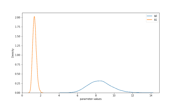
Based on the supplied data, our prior distributions of b0 and b1 have been substantially updated. The two distributions now indicate what the parameters are most likely given both your priors and the observed real data. Now with high confidence in all countries combined b1 (price-sensitivity) is likely between 1 and 2, while b0 is between 6 and 11. This allows us to perform some inference and already implies a valuable result: Virtuoso’s clients seem very unlikely to accept prices above 13, while prices under 10 would have at least a 50% chance of being accepted. Unlike other modeling approaches, Bayesian modeling produced whole distributions of acceptance likelihoods for various prices that would allow us to directly take uncertainty into account when making difficult decisions.

We can also directly use this model for traditional forecasting and estimate its accuracy (and other metrics). We have previously split the full dataset into a 2-to-1 train-test split, and only training data has been supplied to PyMC3. Now we can directly access all available posterior values from this model (using ‘posterior’ variable) to further make predictions for various prices. While PyMC3 has built-in methods to do so, it is more illustrative to reconstruct probabilities ourselves. If we do want a point-estimate, we can infer a single property of each posterior distribution such as the mean. As seen in Figure 1, the mean of b0 is 8.5 and of b1 is 1.3. Consequently, for a price of 5 this would translate into logit(8.5 – 1.3 5) = 0.85 where logit is the standard logit function. In other words, a price of 5 implies a 85% chance to be accepted in each country on average. Similarly, we can calculate probabilities for each of the X_test prices, convert them to 1 or 0 (e.g. based on a standard 0.5 threshold) and compare them to the real y_test values. As a result, this pooled Bayesian model* has an accuracy of 85.4% as well as a weighted f1-score of 85%, which can be further improved if we change aspects such as the chosen probability threshold or the posterior statistics (e.g. use some quantile value like the median rather than the mean).

A hierarchical framework

We can do even better than this. So far, we have pooled all country data together, constraining ourselves to only learn the ‘average truth’. But Bayesian modeling particularly shines when we let it handle several distinct yet related problems together. Such frameworks are usually referred to as ‘hierarchical’ – we assume that there is a certain hierarchy and common logic in how people react to our prices in different countries. These reactions are probably similar yet somewhat different. We can incorporate this idea into our Bayesian model by assuming that our three countries have different b0 and b1, that are related by being generated by common distributions. It may sound tricky, but consider the following simplified example:

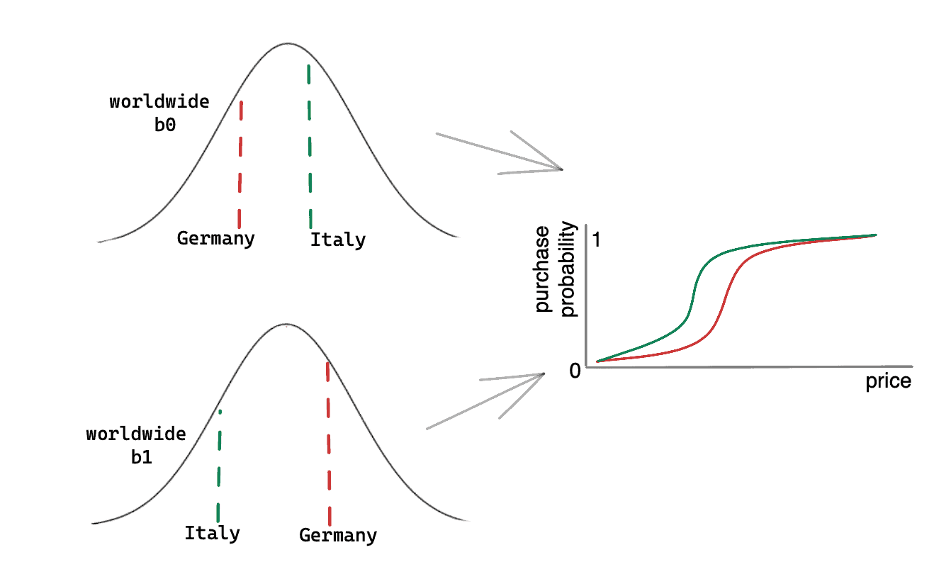
In this example there are only Germany and Italy. Both have different likelihoods of purchasing at each price, as illustrated by the logistic curves in the rightmost plot. We already saw that we need two parameters for each of these curves: b0 and b1. Here they are different for each country, but they come from common distributions (on the left). It is much like saying that there are different price-sensitivities in countries worldwide, distributed like shown in the bottom-left plot. Germany and Italy may have different parameters, but those parameters share common origin.

You may wonder how we could know these common worldwide distributions. Actually, we do not. But we can also determine what they could look like while solving the Bayesian problem as a whole! By having data from multiple countries, we can learn about the problem as a whole. This can later also inform us about the countries we have not even seen before or where we have very little data.

So, by adopting this hierarchical framework, we do not have to assume that Italy, Germany, and France are the same, but we also do not assume that they have nothing in common. As a result, such models learn the differences, while acknowledging the similarities present in the data. This presents a valuable middle ground that other modeling approaches rarely can provide. In terms of code, our extended model takes this form:

with pm.Model() as hier_model:

    # priors for common distribution's mu and sigma
    mu_b0 = pm.Normal('mu_b0', mu=0, sd=100)
    mu_b1 = pm.Normal('mu_b1', mu=0, sd=100)

    sigma_b0 = pm.InverseGamma('sigma_b0', alpha=3, beta=20)
    sigma_b1 = pm.InverseGamma('sigma_b1', alpha=3, beta=20)

    # country-specific draws 
    b0 = pm.Normal('b0', mu=mu_b0, sd=sigma_b0, shape=n_countries)
    b1 = pm.Lognormal('b1', mu=mu_b1, sd=sigma_b1, shape=n_countries)

    # compute the purchase probability for each case
    logit_p = b0[ids_train] - b1[ids_train] * X_train['price']
    likelihood = pm.Bernoulli('likelihood', logit_p=logit_p, observed=y_train)

    posterior = pm.sample(draws = 10000, tune = 5000, target_accept = 0.9)

This model may look more complicated, but in fact it is built around an idea very similar to the previous pooled model. Again, Bernoulli likelihood combines the observed y_train data with the logistic probabilities that combine b0 and b1 (this time different yet related for each country). Each b0 and b1 still comes from the same type of prior distributions as before but now not fixed ones but ‘flexible’ distributions with unknown mu and std. These mu and std all have priors of their own as previously illustrated in Figure 2. Those new additional priors are very generic (uninformed) as we do not have a good idea how mu and std are distributed worldwide. A normal distribution around zero with a large std is a common choice in this case. Finally, we need to assign an index to each country and insert it into probability definitions to let PyMC3 use the correct betas for each country. This ids_train variable must have the same order of countries as prices in X_train.

Now we are again ready to generate posterior distribution samples using MCMC. When it succeeds, we can inspect the unique parameter distributions generated for each country:

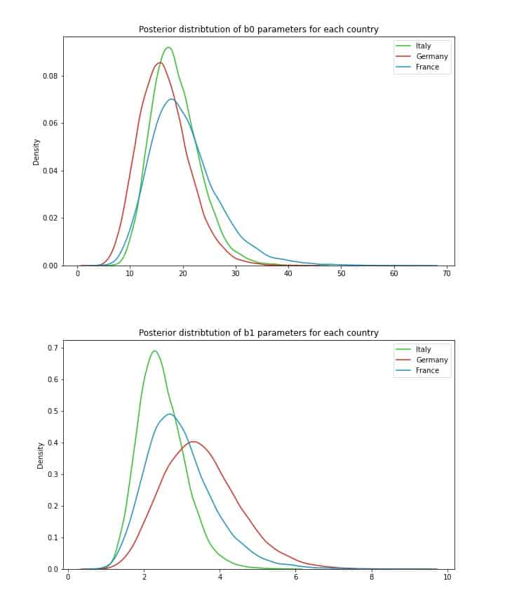
While all *b0* seem very similar, there is some more noticeable distinction in *b1* parameters. This makes practical sense – *b1* indicates how sensitive clients in each country are to price increases, and the posterior with the highest mean is the one for Germany – where Virtuoso had by far the lowest fraction of accepted offers. By contrast, Italy, where sales were the highest, appears to be least sensitive to price increases. Furthermore, the width of each distribution is also informative. Broader width indicates more uncertainty – we may want to experiment a bit more in Germany to get a better idea of a good price strategy there. This is a rather unique advantage of the hierarchical Bayesian framework – together with the forecasting model we gain diverse analytical information about the problem we are dealing with.

Now that we know price sensitivity in each country, we can compare various pricing strategies. Let’s say Virtuoso wants to set a fixed price of 7 for all clients and offer a (temporary) discount of 2 for (more price-sensitive) clients in Germany. We can calculate not just point estimates but whole probability distributions for price acceptance of clients in each country:

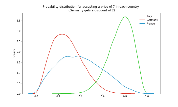
Interestingly, while German clients have their price reduced to 5, they are still the least likely to purchase our services (with a mean of ~20%). Perhaps a higher discount was necessary? By contrast, Italian clients are more than 80% likely to accept their price of 7.

Not only mean values are valuable here though: we can also infer that the probability distribution of France at these prices is by far the most uncertain one. Knowing uncertainty around our predictions (big advantage of Bayesian modeling), provides us with additional valuable information: one may prefer a less profitable regional client if it yields less uncertainty. Or one can experiment more with the French clients to gather more data and reduce this uncertainty. These are just a few valuable analytical insights that this framework can provide!

Finally, we can see by how much the predictive strength of our model has improved now that we added a hierarchical structure. A few calculations like those we did before show an accuracy of 93.8% and a weighted f1-score of 94%. Therefore, this new structure most certainly improved the overall forecasting performance of our model.

Conclusions

As we have seen so far, Bayesian modeling is not just some fancy confusing concept that statisticians use to scare freshmen. It is a flexible and powerful framework that provides substantial advantages over more ‘traditional’ approaches. With it, we can add more transparency, direct domain knowledge and/or educated assumptions right into the model. And even if we were somewhat wrong, real-world data adjusts all this via Bayes’ theorem, leaving us with a more realistic understanding of the problem at hand, and a usable forecasting framework. Furthermore, it quantified uncertainty and provided valuable analytical insights on top of this all.

This use case has taught us several important practical lessons in its turn. There were several factors that made constructing a Bayesian model (using PyMC3) successful. First, we had to make several decisions regarding the amount of complexity that we want our model to address (such as combining cases/countries together, treating sales as binary events etc.). Second, a careful selection of prior parameter values was necessary (that incorporates our believes and domain knowledge and does not unnecessarily restrict the model). Then, we had to combine it all in an appropriate likelihood function with the real data supplied to it. Finally, we acquired posterior samples using PyMC3’s automated MCMC sampling algorithm. And voila – an accurate and informative Bayesian model is at our service.

Carefully following these steps, as well as gaining more practical experience with the Bayesian framework, will make it a powerful and convenient tool, that would often beat competing approaches or help us when no alternatives are even available.

Check our Bayesian Modeling Training